What each tool exports, drawn by the tool itself on its sample dataset and laid out the way it would sit in a report appendix: numbered, captioned, black on white. Nothing here is retouched. Open any tool to make the same figure from your own data.
Structural geology
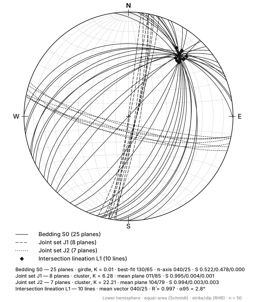
Figure 1. Stereonet. Plot planes, poles and lineations on an equal-area or equal-angle net, with contouring. Open the tool
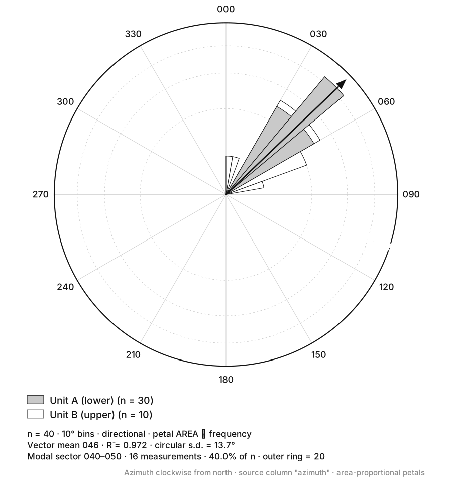
Figure 2. Rose Diagram. Turn a column of azimuths into a directional rose, with adjustable bin width and unidirectional or bidirectional petals. Open the tool
Composition & classification
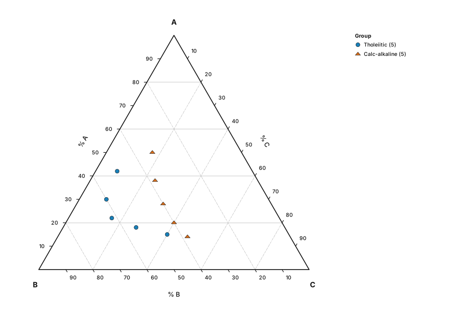
Figure 3. Ternary Diagram. A blank three-component triangle for any composition data — label the apices yourself. Open the tool
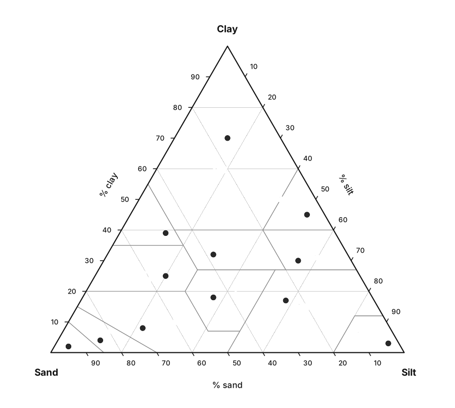
Figure 4. Soil Texture Triangle. Drop sand/silt/clay percentages onto the USDA triangle and read off the texture class. Open the tool
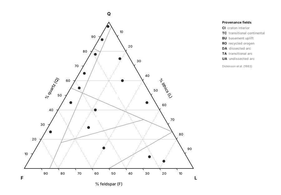
Figure 5. QFL Diagram. Quartz–Feldspar–Lithics point counts on the Dickinson provenance fields. Open the tool
Water chemistry
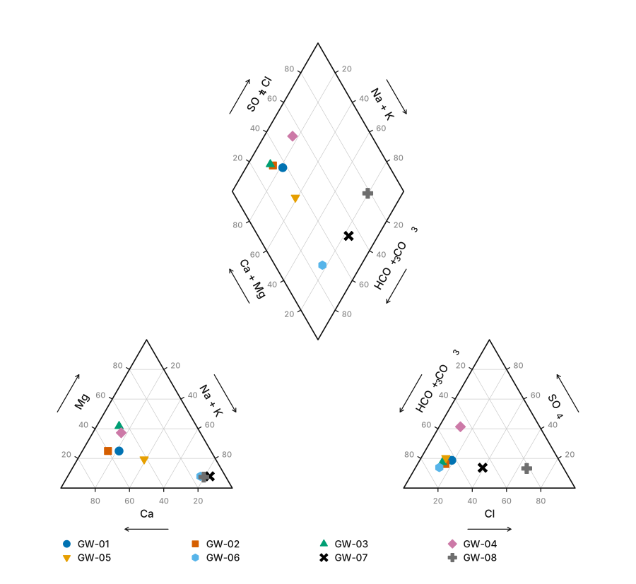
Figure 6. Piper Diagram. Classify water types from major-ion chemistry on the classic Piper trilinear plot. Open the tool
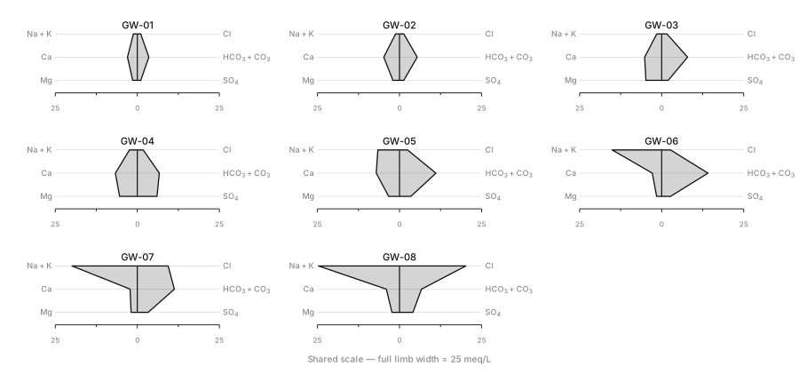
Figure 7. Stiff Diagram. One polygon per sample — the fastest way to see a chemistry change along a flow path. Open the tool
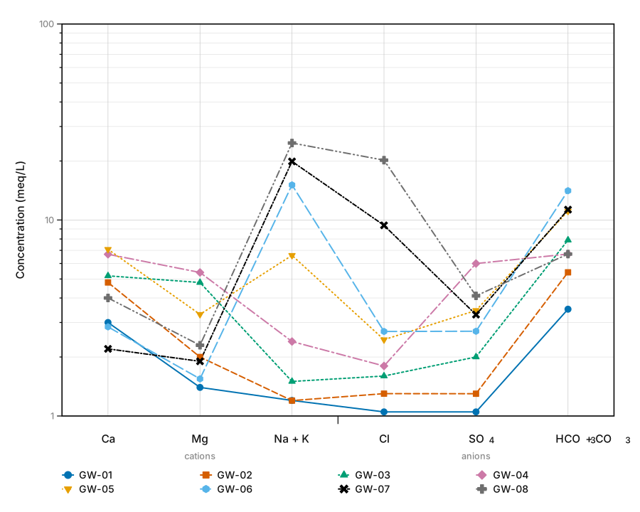
Figure 8. Schoeller Diagram. Semi-log multi-ion profiles that compare absolute concentrations across many samples at once. Open the tool
Geotechnical
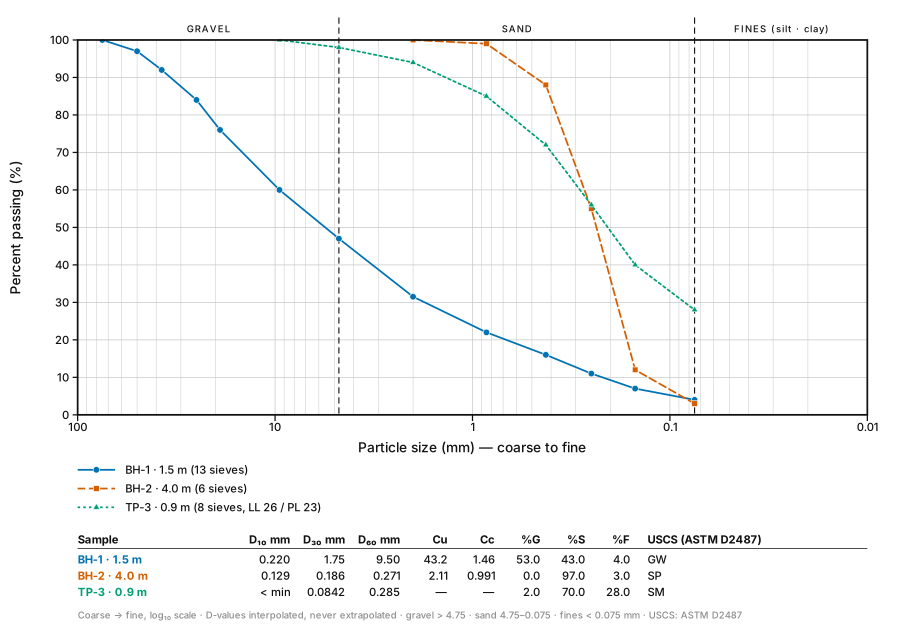
Figure 9. Grain Size Distribution. Turn sieve and hydrometer results into a semi-log particle-size distribution curve, with D10, D30, D60, Cu and Cc read off for you. Open the tool
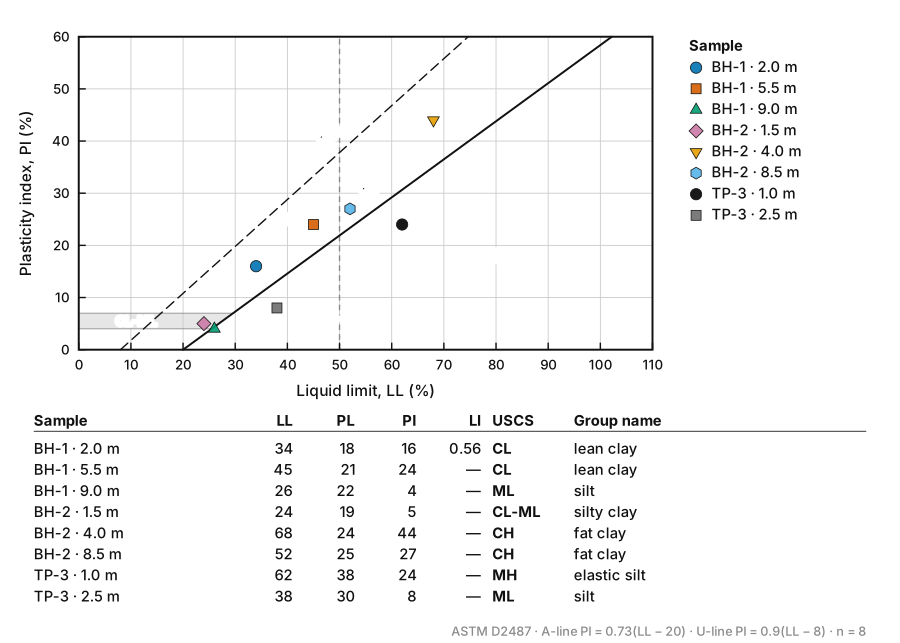
Figure 10. Plasticity Chart. Plot liquid limit against plasticity index on the Casagrande chart, with the A-line and U-line drawn and the USCS group symbol read off. Open the tool
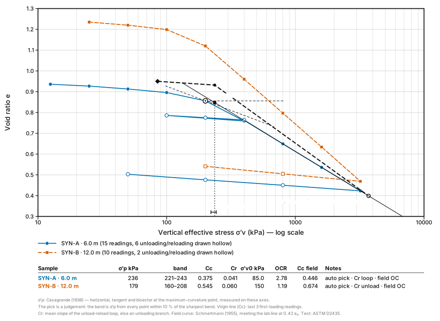
Figure 11. Consolidation Curve. Plot oedometer results as void ratio against log effective stress and find the preconsolidation stress by Casagrande’s construction — with the pick drawn and adjustable, Cc, Cr and OCR worked out, and the Schmertmann field curve. Open the tool
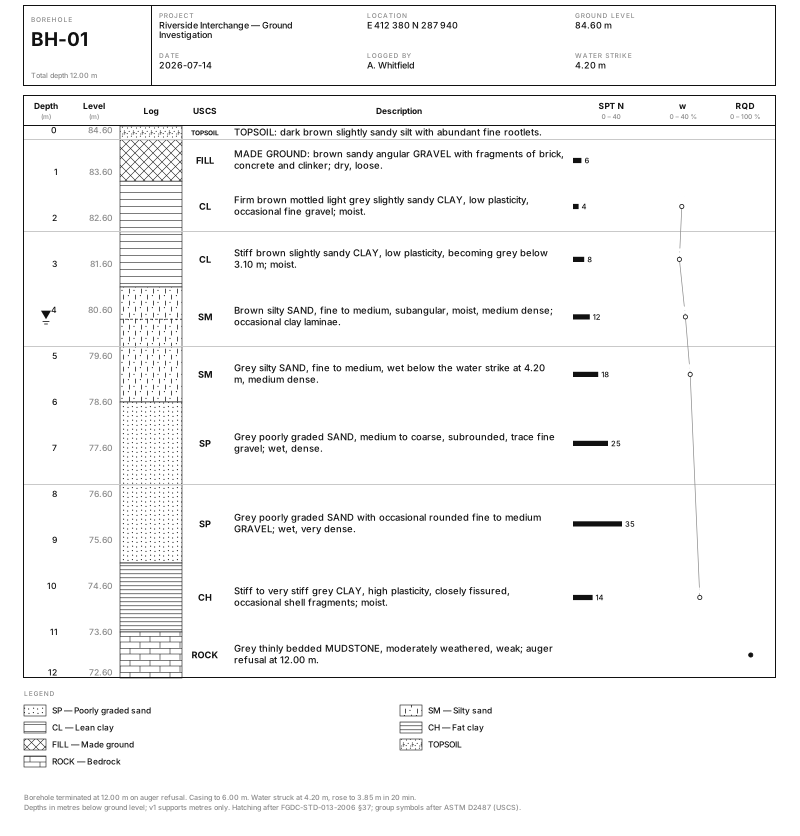
Figure 12. Borehole Log. Turn a table of depth intervals into a publication-ready borehole strip log with USCS hatch patterns, SPT N-values and a water table. Open the toolPro, locked
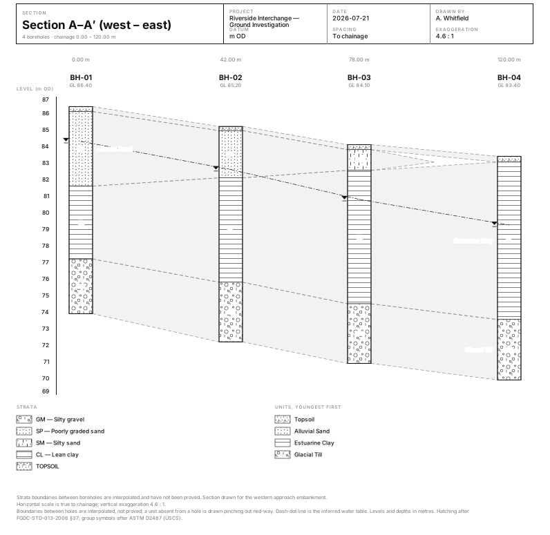
Figure 13. Borehole Correlation. Draw several borehole logs side by side at true elevation and correlate the strata between them, with pinch-outs, a water table and the vertical exaggeration stated. Open the toolPro, locked
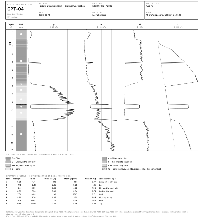
Figure 14. CPT Profile. Turn a cone penetration test file into a publication-ready sounding profile — qc, fs, Rf and u2 tracks on one depth axis, with a Robertson (1986) soil behaviour type strip and an interpreted layer table. Open the toolPro, locked
Rock & Tunnel
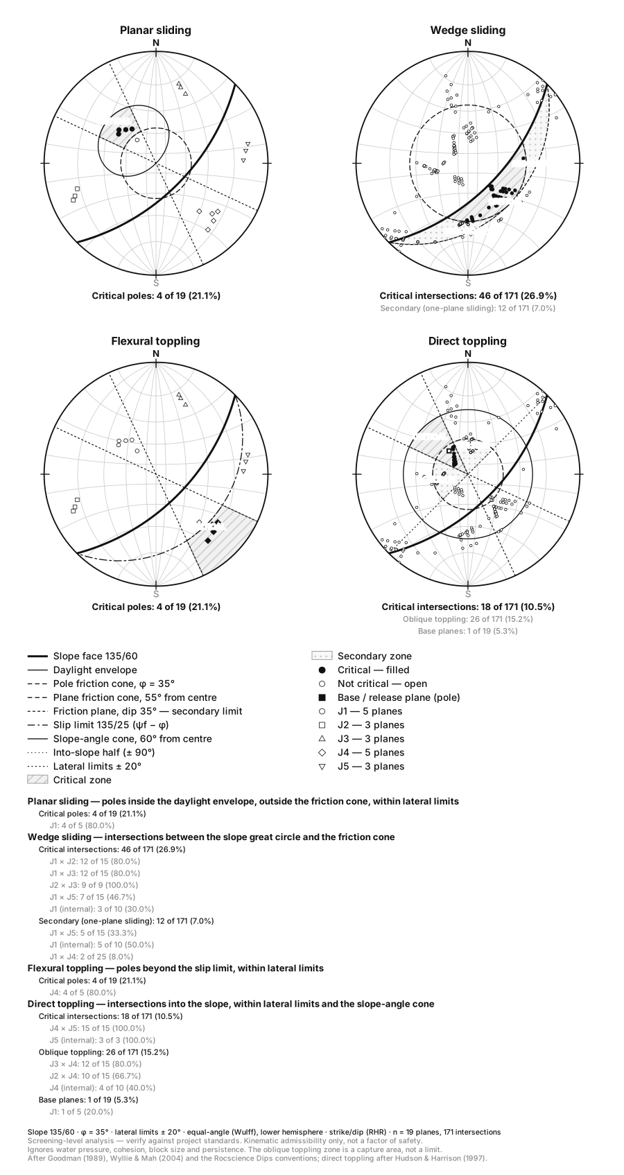
Figure 15. Kinematic Analysis. Screen a rock cut for planar sliding, wedge sliding and toppling on a stereonet, with the daylight envelope, friction cone, lateral limits and slip limit drawn and the critical measurements counted. Open the toolPro, locked
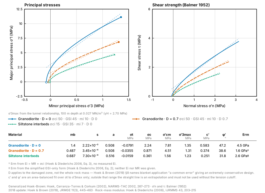
Figure 16. Hoek-Brown Envelopes. Generate Generalized Hoek-Brown strength envelopes from σci, GSI, mi and D — with mb, s, a, the tensile cutoff, rock-mass strength, the equivalent Mohr-Coulomb c′ and φ′ and the rock-mass modulus worked out and cited. Open the tool
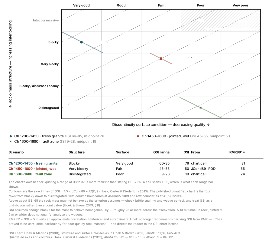
Figure 17. GSI Chart. Plot your rock-mass descriptions on the Geological Strength Index chart — blockiness against surface condition, the diagonal GSI contours drawn, and a range rather than a false decimal for every scenario. Open the tool
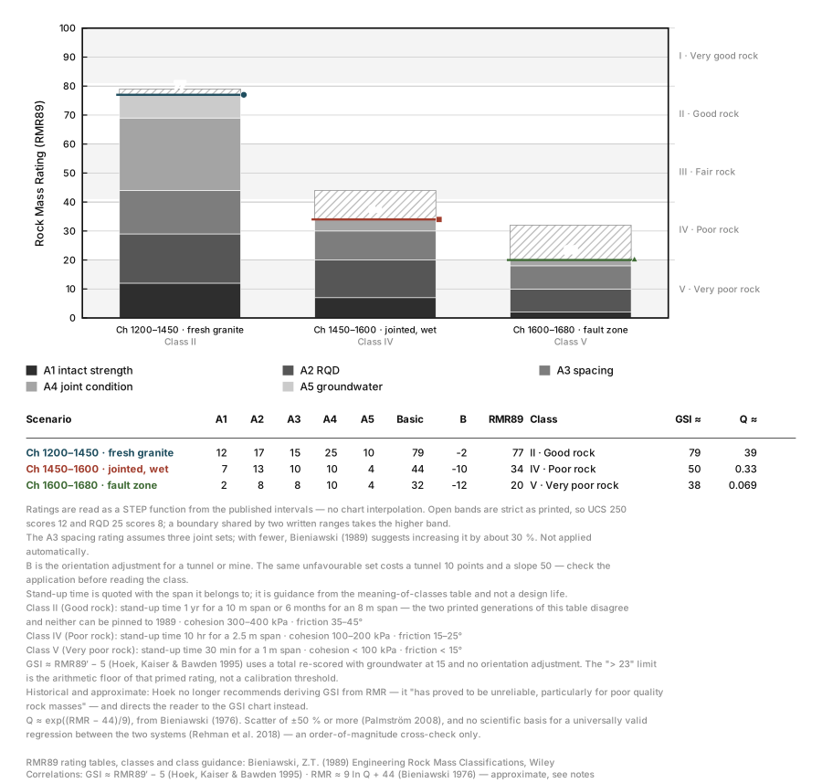
Figure 18. RMR Calculator. Work out Bieniawski (1989) RMR89 from the five published rating tables plus the orientation adjustment — with the rating breakdown drawn as a stacked bar against the class I–V bands, and the GSI and Q correlations printed and cited. Open the tool
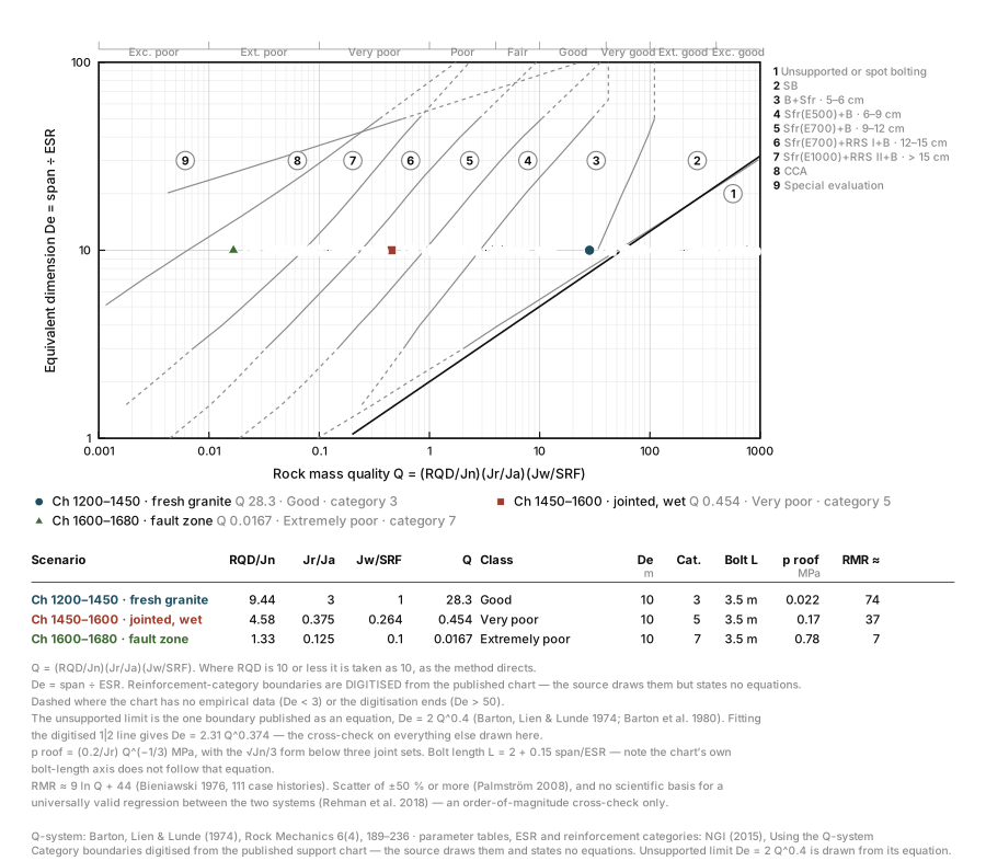
Figure 19. Q-System Calculator. Compute Barton’s Q from RQD, Jn, Jr, Ja, Jw and SRF, then read the support requirement straight off the NGI chart — Q against equivalent dimension, with the nine reinforcement categories drawn and your scenarios plotted on them. Open the tool
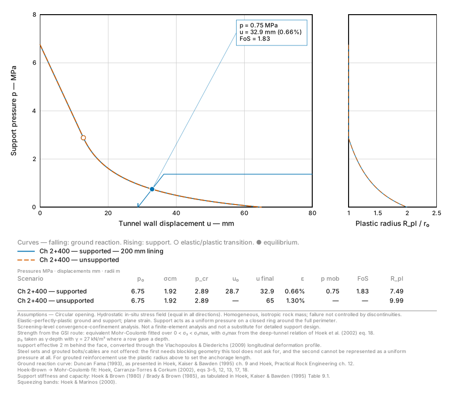
Figure 20. Ground Reaction Curve. Draw the ground reaction curve, the support characteristic curve and the equilibrium between them for a circular tunnel — with the mobilised support pressure, factor of safety, plastic zone radius and tunnel strain read straight off the figure. Open the toolPro, locked
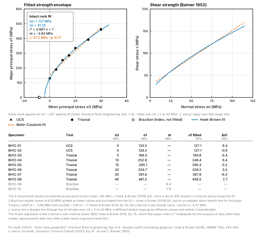
Figure 21. Rock Strength Fitting. Fit the Hoek-Brown intact constants σci and mi to triaxial test data by Hoek’s published linear regression, with r², a Mohr-Coulomb c′ and φ′ over the tested range, the tension cutoff and every specimen’s residual. Open the tool
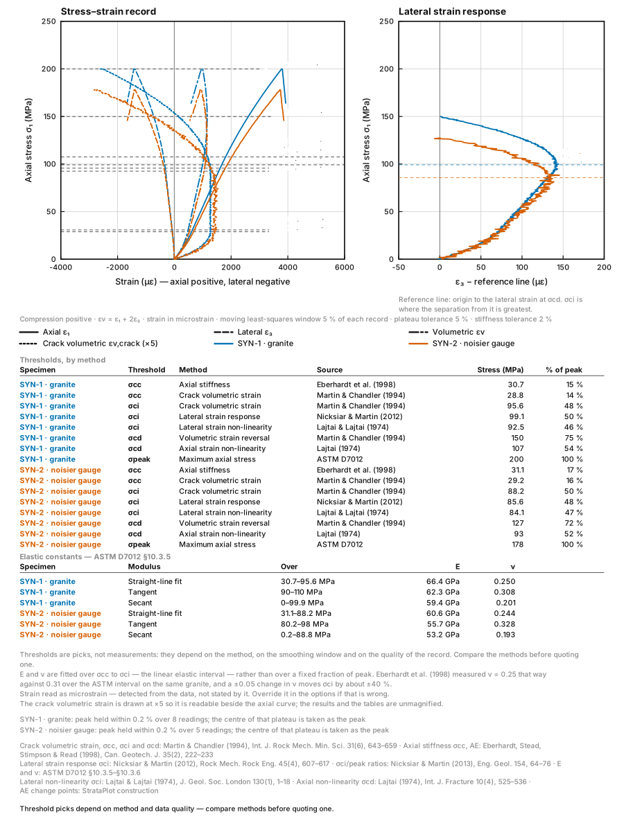
Figure 22. Crack Thresholds. Pick crack closure, crack initiation, crack damage and peak stress off a uniaxial or triaxial stress–strain record by several published methods at once — with the crack volumetric strain, the lateral strain response, E and ν worked out and every method cited. Open the tool
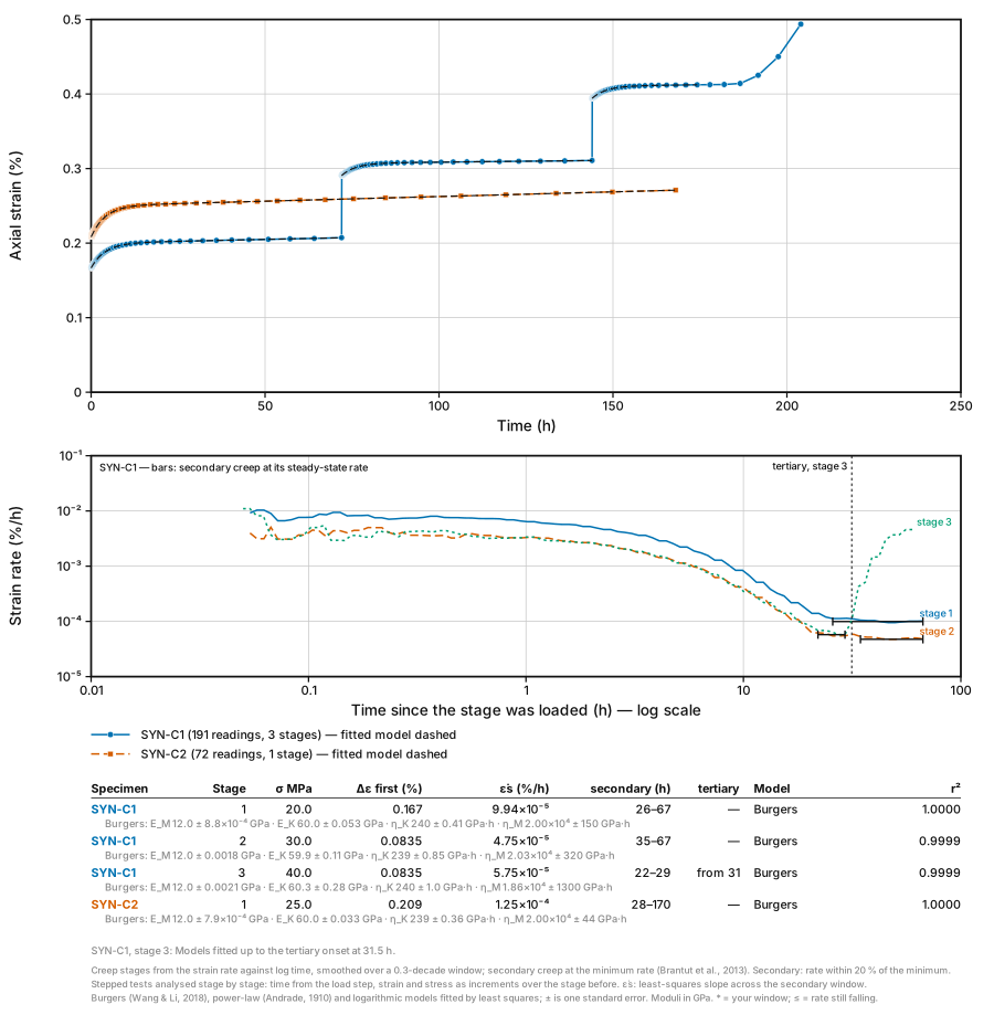
Figure 23. Creep Test Analysis. Analyse a creep test stage by stage: strain and strain rate against time, primary, secondary and tertiary creep found from the rate, the steady-state creep rate, and Burgers, power-law and logarithmic fits compared with their standard errors. Open the toolPro, locked
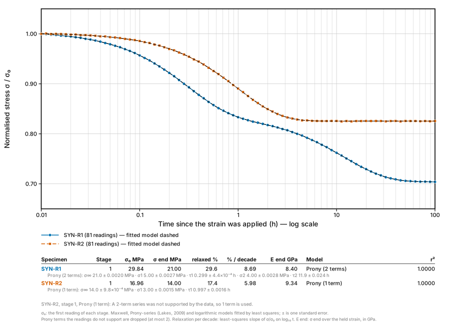
Figure 24. Stress Relaxation. Analyse a stress relaxation test: σ/σ₀ against log time, total relaxation and relaxation per decade, and Maxwell, Prony-series and logarithmic fits compared, with the relaxation modulus when the held strain is given. Open the toolPro, locked