Reading a Grain Size Distribution Curve
A particle size distribution curve compresses a whole sieve analysis into one line, and four numbers read off that line decide how the soil will compact, drain and classify. This is how to read them, with the arithmetic shown.
Updated
The axes, and why one of them is logarithmic
A particle size distribution curve plots percent passing on a linear vertical axis from 0 to 100, against particle diameter on a logarithmic horizontal axis. By convention the diameter axis runs coarse to fine from left to right, so the curve rises from bottom-left to top-right and a steeper curve means a narrower range of sizes.
The logarithmic axis is not a stylistic choice. A single soil routinely spans 75 mm cobbles down to 0.001 mm clay — five orders of magnitude. On a linear axis, everything below 1 mm would collapse into the first pixel of the plot, and the fine fraction, which controls permeability and plasticity, would be invisible. On a log axis each decade gets equal width, so a factor-of-two change in diameter looks the same at 20 mm as it does at 0.02 mm.
A consequence follows that trips people up constantly: anything read off this curve must be interpolated logarithmically, not linearly. Straight-line interpolation between two sieve points is straight in log-diameter space, not in diameter space.
Where the data come from
A full curve is usually two tests joined at 0.075 mm.
Sieve analysis — ASTM D6913 or BS 1377-2 — covers everything coarser. A dried, weighed sample is washed free of fines, dried again, and shaken through a nest of sieves of decreasing aperture. Each sieve is weighed, and the retained masses are converted to cumulative percent passing, which is the quantity the curve is defined on.
Hydrometer analysis — ASTM D7928 — covers the fines, because particles below about 75 µm will not sieve reliably at any amount of shaking. A dispersed suspension is left to settle and its density measured over time, and Stokes' law converts settling velocity into an equivalent spherical diameter. That phrase is doing work: a plate-shaped clay particle has no single diameter, so what the hydrometer reports is the diameter of a sphere that would settle at the same rate. A visible step at 0.075 mm means the two halves of the test disagree.
Reading D₁₀, D₃₀ and D₆₀
The three key readings are defined the same way: D₆₀ is the particle diameter at which 60% of the sample by mass is finer, and likewise for D₃₀ and D₁₀. They are read off the curve, not measured in the laboratory — enter the vertical axis at the percentage, go across to the curve, drop down to the diameter axis.
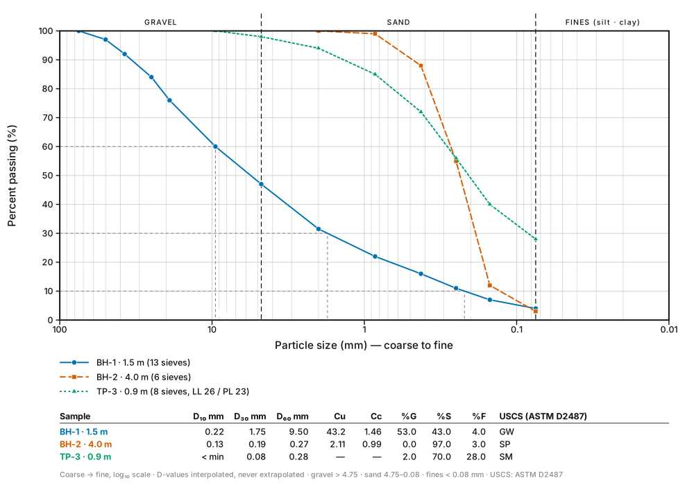
Take BH-1, the broad curve. D₆₀ falls exactly on a sieve: 60% passes the 9.5 mm sieve, so D₆₀ = 9.5 mm with no interpolation needed. D₁₀ does not: the readings straddle it at 0.15 mm (7% passing) and 0.25 mm (11% passing). Interpolating on the log axis:
- Fraction of the interval: (10 − 7) ÷ (11 − 7) = 0.75
- log₁₀ D₁₀ = log₁₀(0.15) + 0.75 × [log₁₀(0.25) − log₁₀(0.15)] = −0.824 + 0.75 × 0.222 = −0.658
- D₁₀ = 10⁻⁰·⁶⁵⁸ = 0.22 mm
The same construction between 0.85 mm (22%) and 2.0 mm (31.5%) gives D₃₀ = 1.75 mm. Doing that last one linearly instead would have returned 1.82 mm — a 4% error that propagates squared into the coefficient of curvature.
D₁₀ carries a name of its own: the effective size. It is called that because the finest tenth of a soil controls its permeability far more than the mean size does — flow is throttled at the narrowest pore throats, and those are set by the small particles filling the gaps between the large ones. Hazen's old approximation, k ≈ C · D₁₀² with D₁₀ in millimetres and k in cm/s, still works as an order-of-magnitude check. For BH-2 at D₁₀ = 0.13 mm and C ≈ 1, that is about 1.7 × 10⁻² cm/s — a freely draining sand. Hazen is only valid for clean sands with D₁₀ between roughly 0.1 and 3 mm and Cu below about 5, which BH-2 satisfies and BH-1, with Cu over 40, emphatically does not.
Cu and Cc: two numbers for the shape of the curve
The three readings feed two dimensionless shape coefficients, and between them they describe the whole curve well enough to classify it.
The coefficient of uniformity, Cu = D₆₀ ÷ D₁₀, measures how wide the range of sizes is. A value near 1 means every particle is nearly the same size — the curve is almost vertical. A large value means the soil spans many decades.
The coefficient of curvature, Cc = D₃₀² ÷ (D₁₀ × D₆₀), measures whether the curve is smooth over that range or has a gap in the middle. If D₃₀ sits where a smooth curve would put it, Cc lands between 1 and 3. If a size fraction is missing, D₃₀ is pulled towards one end and Cc falls outside that window — a gap-graded soil.
For BH-1: Cu = 9.5 ÷ 0.22 = 43.2, and Cc = 1.75² ÷ (0.22 × 9.5) = 3.06 ÷ 2.09 = 1.46.
For BH-2: Cu = 0.27 ÷ 0.13 = 2.11, and Cc = 0.19² ÷ (0.13 × 0.27) = 0.99.
Well graded or poorly graded
The USCS turns those two numbers into a letter, with a different uniformity threshold for gravels and sands:
| Soil | Well graded (W) requires | Otherwise |
|---|---|---|
| Gravel | Cu ≥ 4 and 1 ≤ Cc ≤ 3 | Poorly graded (P) |
| Sand | Cu ≥ 6 and 1 ≤ Cc ≤ 3 | Poorly graded (P) |
BH-1 passes both — Cu 43.2 against a requirement of 4, Cc 1.46 inside the window — and classifies as GW, a well-graded gravel with sand. BH-2 fails on uniformity alone: Cu 2.11 against a requirement of 6, so it is SP, a poorly graded sand, regardless of its perfectly respectable Cc of 0.99.
Note what "poorly graded" does not mean. It is not a quality judgement, and a uniform sand is not a defective soil. It means the curve is steep, and a steep curve is exactly what a filter medium or a drainage layer is specified to have. The term describes the shape of the line, nothing more.
Why the shape matters on site
A well-graded material compacts to a denser, stronger and less permeable fill, because the small particles occupy the voids between the large ones and the whole mass interlocks. That is what a structural fill specification is asking for. A poorly graded material has more void space, a lower maximum dry density and a far higher permeability — undesirable under a foundation, and precisely correct behind a retaining wall or in a drainage blanket. Neither is better; they are for different jobs.
When a D-value cannot be read
The third curve in the figure stops at 28% passing on the 0.075 mm sieve. There is no point on it at 10% passing, so D₁₀ does not exist within the data — and Cu and Cc, which both depend on it, cannot be calculated either.
The correct response is to report them as not determinable. Extrapolating the curve down into the fines to manufacture a D₁₀ is guessing at a value that then propagates into a permeability estimate and a classification. It is also unnecessary: this soil has 28% fines, and under the USCS a coarse soil with more than 12% fines is classified from the plasticity of its fines, not from its gradation. The missing numbers were never going to be used.
The same caution applies at the coarse end. If the largest sieve passes less than 60% of the sample, D₆₀ is off the top of the curve and Cu is undefined — usually a sign that the specimen needed a larger sieve in the stack, or that oversize particles were removed without being accounted for.
Other things the curve is used for
- Filter design. A granular filter must be fine enough to retain the soil it protects and coarse enough to drain it. Terzaghi's criteria are ratios between the filter's D₁₅ and the base soil's D₈₅ and D₁₅ — all read off the same curves.
- Grading envelopes. A fill specification is usually written as an upper and a lower curve rather than a single target, and compliance is checked by plotting the site test on the same axes to see whether it fits between them.
- Liquefaction screening. Uniform, clean, saturated fine sands — steep curves in the 0.075 to 0.85 mm range, with Cu below about 6 — are the classic liquefaction-susceptible gradation.
- Frost susceptibility. Rules of thumb are stated as a percentage finer than 0.02 mm, read directly off the hydrometer end of the curve.
Keep reading
- USCS Soil Classification Explained
The Unified Soil Classification System worked end to end: the group symbols, the decision path with its threshold numbers, when a dual symbol is required, and what the plasticity chart decides.
- How to Read a Stereonet
Stereonets explained: equal-area vs equal-angle projection, great circles vs poles, density contouring, and what a girdle of poles tells you about a fold.